3.5 Model Evaluation and -Selection
Several algorithms (estimators) were trained in parallel. Once good hyperparameters were found using randomized grid search, performance of the estimators was compared using a common metric in order to select the best (see Figure 2.14 for a schematic process overview). This was done independently for classifiers (predicting the binary target) and regressors (predicting the continuous target). The process is documented in notebook 6_Model_Evaluation_Selection.ipynb14.
The pipeline functionality of scikit-learn was used to combine preliminary data transformations, i.e. scaling of features (where necessary) and resampling with the estimator-algorithm. This allows to jointly tune hyperparameters for transformations and the estimator.
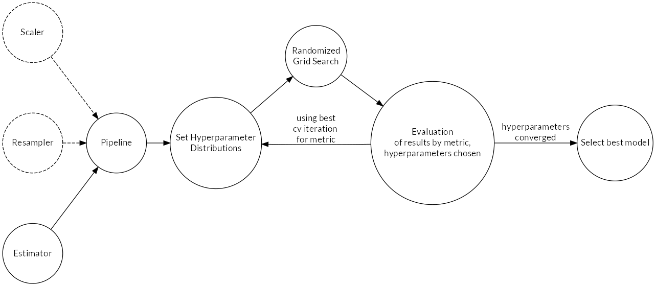
Figure 2.14: Learning process schematic.
A common random seed was used for all algorithms and random number generators.
3.5.1 Evaluation
Randomized grid search was run with 10-fold cross-validation (CV). The best-performing pipeline for each algorithm was stored in a python dictionary during evaluation. The dictionary was persisted to disk and only updated when an algorithm’s metric improved. This ensured that the best hyperparameter settings were always retained during the extensive model evaluation phase.
3.5.1.1 Randomized Grid Search
In randomized grid search, (Bergstra and Bengio 2012), probability distributions for hyperparameter values are specified. The algorithm then runs a defined number (10 were used) of random combinations by sampling from the distributions. Compared to the usual grid search, this can greatly speed up the learning process because good hyperparameter settings are generally identified with less iterations.
After one round of learning, the hyperparameter distributions were adjusted before the next iteration as follows: When the best value was found near the limits of the domain, the distribution was shifted in this direction. For values falling inside the domain, the distribution was narrowed down towards the found value. This procedure was repeated until the hyperparameters converged.
The implementation of randomized grid search in scikit-learn returns a summary table with the CV results for each hyperparameter combination. By comparing the mean test score for the chosen metric, the best hyperparameters can be determined.
3.5.1.2 Cross-Validation
CV splits the training data into several folds of equal size. The algorithm is trained as many times as there are folds, holding back one of the folds at each training step for validation using some specified performance metric and training with the rest of the data. This procedure enables quantification of the generalization error and the calculation of statistics that indicate the variance of the model. Following guidance in Kohavi and others (1995), 10-fold CV was used, which trades higher bias for lower variance compared to fewer folds.
3.5.2 Selection
3.5.2.1 Classifiers
Both recall and F1 were initially selected and calculated during model evaluation. In the end, recall was used to select the best classifier as it produced better estimators for the task. Reasoning for the choice of these metrics is given below.
For classification problems, the confusion matrix (see Figure 2.15) can be used to construct various performance metrics. A true positive (TP) indicates a correctly predicted 1, a false negative (FN) is a falsely predicted 0, a false positive is a falsely predicted 1 and finally a true negative (TN) is a correctly predicted 0.
For the data analyzed here, 1 means an example has donated, 0 means the example has not donated.
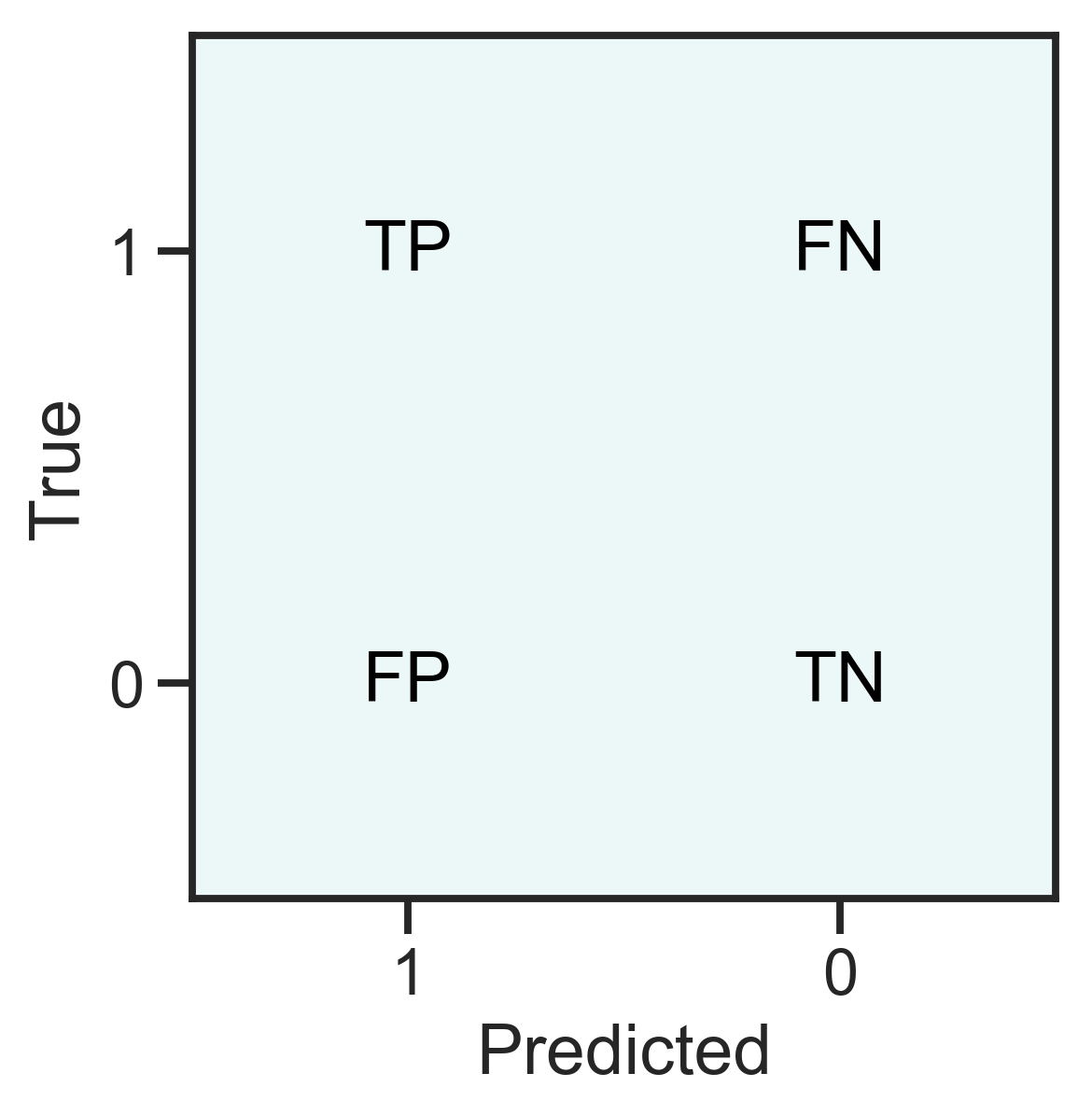
Figure 2.15: Definition of the confusion matrix for a two-class problem.
The definitions of some often-used metrics are given below15. The choice of metric depends on the goal of the prediction and the data at hand.
\[\begin{align*} \text{Recall / Sensitivity / True Positive Rate TPR} &= \frac{TP}{TP + FN} \\ \text{Specificity / True Negative Rate TNR} &= \frac{TN}{TN+FP} \\ \text{Precision / Positive Predictive Value PPV} &= \frac{TP}{TP + FP}\\ \text{Negative Predictive Value NPV} &= \frac{TN}{TN+FN}\\ \text{False Negative Rate FNR} &= \frac{FN}{FN+TP}\\ \text{False Positive Rate FPR} &= \frac{FP}{FP+TN}\\ \text{Accuracy} &= \frac{TP + TN}{TP + FP + FN + TN} \\ \text{F1 score} &= \frac{2TP}{2TP+FP+FN} \end{align*}\]
The goal, as mentioned earlier, is to maximize net profit. To achieve this, a balance between predicting as many TP’s as possible while keeping the number of FP’s low has to be found. One FP costs 0.68 $ (sending a letter to a non-donor). Keeping in mind the distribution of \(\text{TARGET}_D\) (Section 2.2.2), one FN means loosing at least 0.32 $ of possible profit (not sending a promotion to a donor, smallest donation amount is 1 $). The expected loss in profit for one FN is even 15 $ (corresponding to the mean donation amount), which means that with each TP, the cost of 22 FP’s can be covered on average.
The default metric for classification is accuracy, but in the case of imbalanced targets, it is not a desirable metric (TN is present both in the nominator and denominator, dominating the score). The metrics that could be used beneficially because they involve TP an not TN are F1, recall and precision. Since in precision, the FP of the majority class have the highest influence from among the three, it was discarded from the candidate list.
3.5.2.2 Regressors
For regression, \(R^2 = 1- \frac{\sum_{i=1}^n(y_i-\hat{y}_i)^2}{\sum_{i=1}^n(y_i-\bar{y})^2}\) was used, mainly because it is the default metric for regression algorithms in scikit-learn. \(R^2\) has the drawback of depending on the variance of the data used to fit the model and therefore is different for other data. It was however assumed that because learning and test data have the same generating function, \(R^2\) can be used to select a regression model.
3.5.3 Dealing With Imbalanced Data
Several different approaches were explored. The following over-/undersampling techniques available in package imblearn by Lemaître, Nogueira, and Aridas (2017) were studied:
- Random oversampling of the minority class
- Random undersampling of the majority class
- SMOTE (synthetic minority oversampling technique), variant borderline-1
The random sampling algorithms either draw from the minority class with repetition or draw random samples from the majority class without repetition until the labels are balanced. SMOTE does not sample from the data but instead generates synthetic samples from the minority class, thereby countering the danger of overfitting by learning on a small number of repeated observations (random oversampling) or a small subset of the training data available (random undersampling). The SMOTE variant borderline-1 chosen generates samples that are close to the optimal decision boundary, where misclassification is likely.
Additional experiments were run with class- and sample-weights set on the data without resampling. For class weights, the ratio of non-donors vs. donors was used. For sample weights, the donation amount was employed, rescaled to the interval \([0,1]\).
3.5.4 Algorithms
A short introduction of each algorithm is given below. For each algorithm, the hyperparameters that were tuned during learning are given. The choice of algorithms was made so as to cover a wide range of underlying concepts.
3.5.4.1 Random Forest
Random forest (RF) belongs to the family of so-called ensemble learners and was introduced by Breiman (2001). Predictions are made by majority vote of an ensemble of decision trees (CART, Breiman et al. (1984)). The RF can be employed both for regression and classification tasks. RF’s are insensitive towards scale differences in the individual features, and, depending on the implementation, can deal with missing values. Another important feature of RF is the assessment of variable importance by summing the loss improvement for each split in every tree per feature (Friedman, Hastie, and Tibshirani 2001).
During learning, a random sample of the available features is drawn with replacement for each tree (bagging, or bootstrap aggregating, see Breiman (1996)), thereby reducing the variance of the ensemble estimator. Furthermore, splits within a tree are determined again on a random subset of the features. These sources of randomness tend to increase bias of the forest, yet the decrease in variance due to averaging through majority vote outweighs the bias increase Friedman, Hastie, and Tibshirani (2001). Breiman (2001) shows that as the forest grows, the generalization error converges almost surely. This means that random forests are insensitive to overfitting and perform better the more trees are grown.
As explained in Friedman, Hastie, and Tibshirani (2001), trees are grown as follows:
For data with n examples and p features \(D = \{\{x_i,y_i\}, i=1 \ldots n, x_i=\{x_{i,1}, x_{i,2}, \ldots x_{i,p}\}\}\), the CART algorithm decides on the structure of the tree, the splitting features and the split points. As a result, the data is partitioned into \(M\) regions \(R_1, R_2, \ldots, R_M\).
Regression The response \(\hat{y}\) is modeled as a constant \(c_m\) for each region: \[\begin{equation} f(x) = \sum_{m=1}^M c_m\mathbb{1}(x \in R_m) \tag{2.5} \end{equation}\]
Using as loss criterion the sum of squares \(\sum_{i=1}^n (y_i - f(x_i))^2\), the best \(\hat{c}_m\) is the average of \(y_i\) in the region: \[\begin{equation} \hat{c}_m=ave(y_i|x_i \in R_m). \tag{2.6} \end{equation}\]
The algorithm greedily decides on the best partition. Starting with all data, a splitting feature \(j\) and a split point \(s\) is considered, creating two regions \(R_1(j,s) = \{X|X_j \leq s\}, R_2(j,s) = \{X|X_j > s\}\). Feature \(j\) and split point \(s\) are chosen by solving \[\begin{equation} \min_{j,s}\left[\min_{c1} \sum_{x_i \in R_1(j,s)}(y_i-c_1)^2 + min_{c2} \sum_{x_i \in R_2(j,s)}(y_i-c_2)^2\right] \tag{2.7} \end{equation}\] with the inner minimization solved using (2.6).
Classification For a binary classification problem with outcomes \(\{0,1\}\), predictions are made through the proportion of the positive class in a region \(R_m\) with \(N_m\) examples \(x_i\) inside, which is given by: \[\begin{equation} \hat{p}_m = \frac{1}{N_m} \sum_{x_i \in R_m} \mathbb{1}(y_i = 1) \tag{2.8} \end{equation}\]
When \(\hat{p}_m>0.5\), the positive class is chosen.
The loss is described by impurity. When making a split, the feature \(j\) resulting in the highest impurity decrease is selected. Impurity is measured by the Gini index. For binary classification: A node \(m\), representing region \(R_m\) with \(N_m\) observations has as proportion of the positive class \(\hat{p}_m = \frac{1}{N_m} \sum_{x_i \in R_m} \mathbb{1}(y_i = 1)\). The Gini index is then defined as \(2p(1-p)\). So the decision function is: \[\begin{equation} \min_{j,s}(\min_{Gini_l} \hat{p}_l + \min_{Gini_r} \hat{p}_r) \tag{2.9} \end{equation}\] for regions \(R_l, R_r\) below the node.
The RandomForestClassifier and RandomForestRegressor included in scikit-learn were used for learning.
Hyperparameters
max_depth, \(\{1,2,3, \ldots\}\): depth of the trees, \(2^n\) leafs maximum. Controls tree size.min_samples_split, \(\{2,3,4,\ldots\}\): Minimum number of samples required to split a node, controls tree size.max_features, \(\{1, 2, \ldots, m\}\): Maximum number of the \(m\) features to consider when searching for a split. Friedman, Hastie, and Tibshirani (2001) recommend values in \(m = \{1, 2, \ldots \sqrt{m}\}\), but for high dimensional data with few relevant features, larger \(m\) can lead to better results because the probability of including relevant features increases.n_estimators, \(\{1, 2, \ldots\}\): Number of trees to grow. In combination with early stopping, this can be set to a high value since learning will stop when the loss converges.class_weight\(\{\text{balanced}, 1,2,\ldots\}\): Weights on target classes: “balanced” calculates weights according to class frequencies, integer values specify weight on majority class relative to minority
3.5.4.2 Gradient Boosting Machine
The main idea behind boosting is to sequentially train an ensemble of weak learners which on their own are only slightly better than a random decision. The predictions of the individual weak learners are then combined into a majority vote (Kearns 1988).
Gradient boosting machine (GBM) extends on this idea. Like a random forest, GBM learns an ensemble of decision trees. However, trees are learned in an additive manner. At each iteration, the tree that improves the model most (i.e. in the direction of the gradient of the loss function) is added. For this thesis, the package XGBoost by Chen and Guestrin (2016) was used. They describe the algorithm as follows:
Assume a data set with \(n\) examples and \(p\) features: \(D = \{\{x_i,y_i\}, i=1\ldots n, x_i=\{x_{i,1}, x_{i,2}, \ldots x_{i,p}\}\}\). The implementation uses a tree ensemble with \(K\) regression trees to predict the outcome for an example in the data by summing up the weights predicted by each tree:
\[\begin{equation} \hat{y}_i = \phi(x_i) = \sum_{k=1}^K f_k(x_i), f_k \in F \tag{2.10} \end{equation}\]
where \(F = \{f(x) = w_{q(x)}\} (q: \mathbb{R}^m \rightarrow T, w \in \mathbb{R}^T)\) is the space of regression trees. \(T\) is the number of leaves in a tree, \(q\) is the structure of each tree, mapping an example to the corresponding leaf index. Each tree \(f_k\) has an independent structure \(q\) and weights \(w\) at the terminal leafs.
For growing the trees in \(F\), the following loss function is minimized:
\[\begin{equation} L(\phi) = \sum_{i=1}^n l(y_i, \hat{y_i}) + \sum_k^K \Omega(f_k) \tag{2.11} \end{equation}\]
Here, \(l\) is a differentiable, convex loss function that measures the difference between predictions and true values. Since \(l\) is convex, a global minimum is guaranteed. \(\Omega(f) = \gamma T + \frac{1}{2}\lambda||w||^2\) is a penalty on the complexity of the trees to counter over-fitting. The algorithm thus features integrated regularization.
Now, at each iteration \(t\), the tree \(f_t\) that improves the model most is added. For this, \(f_t(\mathbf{x_i})\) is added to the predictions at \(t-1\) and compute the loss:
\[\begin{equation} L^{(t)} = \sum_{i=1}^n l(y_i, \hat{y_i}^{t-1} + f_t(\mathbf{x_i})) +\Omega(f_t) \tag{2.12} \end{equation}\]
To find the best \(f_t\) to add, the gradients finally come into play. With \(g_i\) and \(h_i\) the first- and second-order gradient statistics of \(l\), the loss function becomes:
\[\begin{equation} \tilde{L}^{(t)} = \sum_{i=1}^n l(y_i, \hat{y_i}^{t-1} + g_if_t(x_i) + h_i f_t^2(x_i)) +\Omega(f_t) \tag{2.13} \end{equation}\]
Hyperparameters
learning_rate, \([0, 1]\): Shrinkage, decreases step size for the gradient descent when \(\eta < 1.0\), helping convergence. The number of estimators \(f_k\) has to be increased for small learning rates in order for the algorithm to converge.min_child_weight, \([0, \inf)\): Minimum sum of weights of the hessian in a node. When close to zero, the node is pure. Controls regularization.subsample, \([0, 1]\): A random sample from the \(n\) examples of size \(s, s < n\) is drawn for each iteration, countering overfitting and speeding up learning.colsample_by_tree, \([0, 1]\): A random sample of the \(m\) features is drawn for growing each tree.n_iter_no_change, \(\{0,1,2,3, \ldots\}\): Early stopping. Based on an evaluation set, learning stops when no improvement on the performance metric (misclassification error was chosen) is made for a fixed number of steps.
3.5.4.3 GLMnet
The GLMnet is an implementation of a generalized linear model (GLM) with penalized maximum likelihood by Hastie and Qian (2014). Regularization is achieved through \(L^2\) (ridge) and \(L^1\) (lasso) penalties or their combination known as elastic net (Zou and Hastie 2005).
The loss functions are described in Hastie and Qian (2014). For the binary classification task at hand, a logistic regression was performed. The logistic regression model for a two-class response \(G = \{0,1\}\) with target \(y_i = \mathbb{1}(g_i=1)\) is:
\(P(G=1|X=x) = \frac{e^{\beta_0+\beta^Tx}}{1+e^{\beta_0+\beta^Tx}}\) or, in the log-odds transformation: \(log\frac{P(G=1|X=x)}{P(G=0|X=x)}=\beta_0+\beta^Tx\).
The GLMnet loss function for logistic regression:
\[\begin{equation} \min_{\beta_0,\beta} \frac{1}{N} \sum_{i=1}^{N} w_i l(y_i,\beta_0+\beta^T x_i) + \lambda\left[(1-\alpha)||\beta||_2^2/2 + \alpha ||\beta||_1\right] \tag{2.14} \end{equation}\]
where \(w_i\) are individual sample weights, \(l(\cdot)\) the (negative) log-likelihood of the parameters \(\mathbf{\beta}\) given the data, \(\lambda\) the amount of penalization and \(\alpha \in [0,1]\) the elastic net parameter, for \(\alpha=0\) pure ridge and for \(\alpha=1\) pure lasso.
For the regression task, a gaussian family model was used, having loss function:
\[\begin{equation} \min_{(\beta_0, \beta) \in \mathbb{R}^{p+1}}\frac{1}{2N} \sum_{i=1}^N (y_i -\beta_0-x_i^T \beta)^2+\lambda \left[ (1-\alpha)||\beta||_2^2/2 + \alpha||\beta||_1\right] \tag{2.15} \end{equation}\]
where \(l()\) the (negative) log-likelihood of the parameters \(\mathbf{\beta}\) given the data, \(\lambda\) the amount of penalization and \(\alpha \in [0,1]\) the elastic net parameter, for \(\alpha=0\) pure ridge and for \(\alpha=1\) pure lasso.
For learning, GLMnet evaluates many different \(\lambda\) values for a given \(\alpha\) through cross validation. Because GLMnet is sensitive to scale differences in the features, input data (features and target) should be transformed to mean zero and unit variance.
Hyperparameters
n_splits, \(\{3,4,5, \ldots\}\): Number of CV-splits. Typical values are 3, 5 and 10.- \(\alpha\), \([0, 1]\): parametrizes the elastic net. For \(\alpha = 0\) pure ridge, for \(\alpha = 1\) pure lasso.
scoring: Scoring method for cross-validation (log-loss, classification error, accuracy, precision, recall, average precision, roc-auc)
3.5.4.4 Multilayer Perceptron
The multilayer perceptron (MLP) is a so-called feed-forward neural network. The network consists of at least three layers: an input layer, an arbitrary number of hidden layers and an output layer. Each layer is made up of units. The term feed-forward means that information flows from the input layer through intermediary steps and then to the output. The goal is to approximate the function \(f^*\). For a classifier, \(y = f^*(x)\) maps an example \(x\) to a category \(y\). A feed-forward network defines a mapping \(y=f(x, w)\) and learns the weights \(w\) by approximating the function \(f\) (Goodfellow, Bengio, and Courville 2016).
For a binary classification problem on a dataset with \(n\) examples and \(p\) features \(D = \{\{x_i, y_i\}\}, x_i = \{x_{i,1},x_{i,2},\ldots,x_{i,p}\}, y_i \in \{0,1\}, i = 1 \ldots n\}\), the input layer has \(p\) units, the output layer has \(1\) unit. The hidden layers each have an arbitrary number of hidden units.
Each unit, except for the input layer, consists of a perceptron, which is in effect a linear model with some non-linear activation function applied:
\[\begin{equation} y = \phi(w^Tx+b) \tag{2.16} \end{equation}\]
where \(\phi\) is a non-linear activation function, \(w\) is the vector of weights, \(x\) is the vector of inputs and b is the bias. For \(\phi\), typical functions are the hyperbolic tangens \(tanh(\cdot)\), the logistic sigmoid \(\sigma(x) = \frac{1}{1+e^{-x}}\), or, more recently, the rectified linear unit \(relu(x) = max(0,x)\) (Hahnloser et al. 2000; Goodfellow, Bengio, and Courville 2016).
During learning, the training examples are fed to the network sequentially. For each example, the prediction error is calculated using a loss function, which is typically the negative log-likelihood.
Then, the partial derivatives of the loss function with respect to the weights are computed for each unit and the parameters updated using stochastic gradient descent. This process is called back-propagation.
The complete network is a chain of functions, for the network trained here, it is: \[\begin{equation} \mathbf{y} = \phi^{(3)}(\mathbf{W}^{(3)T} \mathbf{\phi}^{(2)}(\mathbf{W}^{(2)T} \mathbf{\phi}^{(1)}(\mathbf{W}^{(1)T} \mathbf{x} + \mathbf{b}^{(1)}) + \mathbf{b}^{(2)}) + \mathbf{b}^{(3)}) \end{equation}\] where \(x\) is the vector of input features, \(y\) is the vector of outputs, \(\mathbf{W}^{(1)}, \mathbf{W}^{(2)}, \mathbf{W}^{(3)}\) are the weight matrices for each layer and \(b^{(1)}, b^{(2)}, b^{(3)}\) are the bias vectors for each layer and \(\phi^{(1)}, \phi^{(2)}, \phi^{(3)}\) are the sets of perceptrons in the corresponding layer.
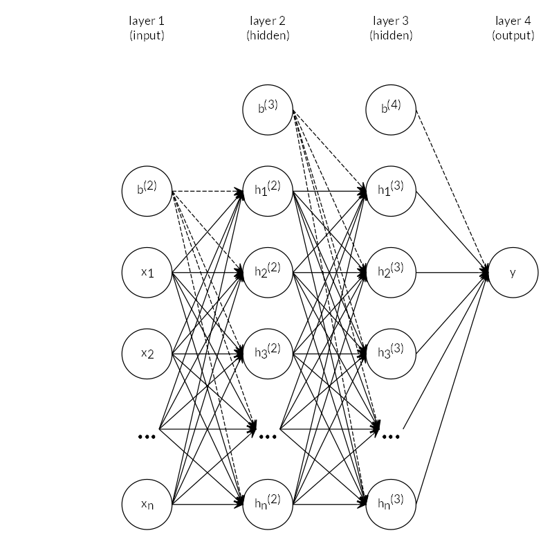
Figure 2.16: Neural network topology used. Two hidden layers \(\mathbf{h^{(1)}, h^{(2)}}\) are contained. \(\mathbf{b^{(2)}, b^{(3)}}\) and \(\mathbf{b^{(4)}}\) are the bias vectors for the respective layers.
For this thesis, the scikit-learn implementation sklearn.neural_network.MLPClassifier was used with default settings (rectified linear unit as activation function, adam (stochastic gradient descent) solver). The network topology was determined by treating it as a hyperparameter. Best results were achieved with a network featuring two hidden layers with 28 hidden units each. The network is shown symbolically in Figure 2.16.
Hyperparameters
hidden_layer_sizes: Tuples, i.e. (100,50,) for a network with 2 hidden layers of 100 and 50 units and one output unit.- \(\alpha\), [0,1]: \(L^2\) regularization amount
learning_rate_init\(>0\): Controls step size for the solver during back-propagation (regularization).
3.5.4.5 Support Vector Machine
In the case of binary classification, support vector classifiers (SVC) find a separating hyperplane \(\{x: f(x)=x^T\beta+\beta_0 = 0\}\) with classification rule \(G(x)=sign(x^T\beta+\beta_0)\). The best hyperplane is such that a margin \(M\) defined by parallel hyperplanes on either side is maximized. The larger the margin, the lower the generalization error. The margin planes contain the examples of the classes that are nearest to each other. In the case of linearly not separable classes (when the classes overlap, see Figure 2.17), a soft-margin SVC may be employed. For examples on the correct side of the hyperplane, the loss is zero. For wrongly classified examples, the loss is proportional to the distance from the hyperplane. A global budget for loss is defined as a constraint and the hyperplane found subject to the constraint (Friedman, Hastie, and Tibshirani 2001).
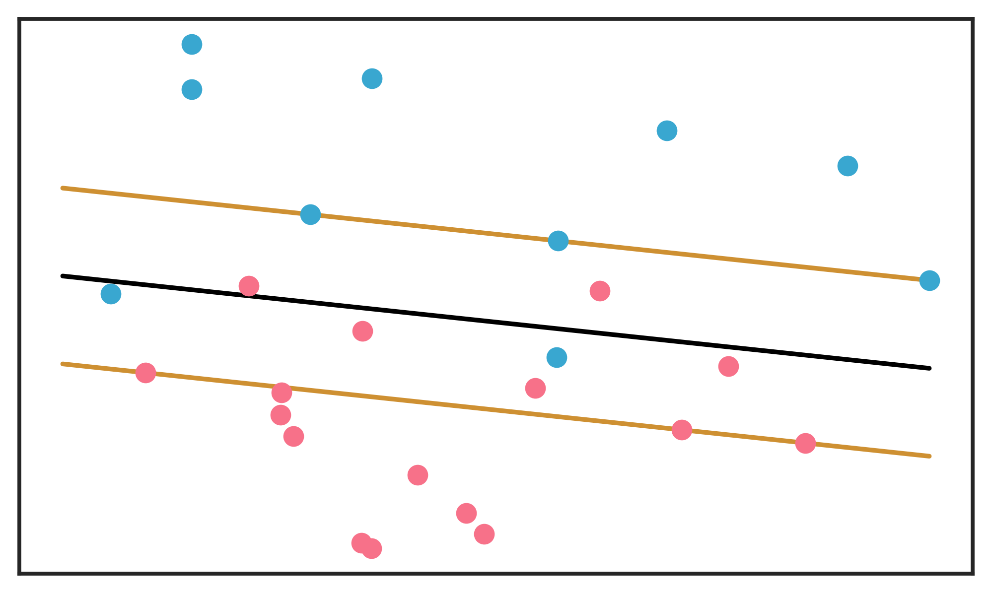
Figure 2.17: Schematic display of an SVM hyperplane (in black), separating two overlapping classes. The margins are shown around the hyperplane, with support vectors falling on the margins. Misclassifications (examples on the wrong side of the hyperplane) have a total budget for distance from the separating plane. The margins are determined by respecting the budget. Adapted from Friedman, Hastie, and Tibshirani (2001).
Support Vector Machines (SVM), (Boser, Guyon, and Vapnik 1992; Cortes and Vapnik 1995) are another approach to the overlapping class case. By mapping the original input space to a high- or infinite-dimensional feature space using nonlinear transformations, a linear hyperplane separating the classes can be found. Calculation of the SVM involves a dot product between the \(x_i\) (Friedman, Hastie, and Tibshirani 2001):
\[\begin{equation} f(x) = \sum_{i=1}^N \alpha_i*y_i\langle h(x), h(x_i)\rangle + \beta_0 \tag{2.17} \end{equation}\]
where \(h(x)\) are the transformations mapping from the input space to the high-dimensional space.
Since the transformations can be prohibitively expensive, the so-called kernel trick (Aizerman, Braverman, and Rozoner 1964) is used (Boser, Guyon, and Vapnik 1992). The trick lies in the fact that knowledge of the kernel function \(K(x,x') = \langle h(x), h(x') \rangle\) suffices, without need to compute the dot products.
Several kernels are possible. In scikit-learn, linear, polynomial, radial basis function and sigmoid are available.
For regression, the Support Vector Regression Machine (SVR) was introduced by Drucker et al. (1997).
scikit-learn implementations were used for both classification and regression.
Hyperparameters
C, \((0,\inf)\): Penalty on the margin sizekernel: One of linear, poly, rbf or sigmoiddegree\(\{1,2, \ldots \}\): Degree of polynomial kernelclass_weight: Automatic balancing or a dictionary with weights per class
3.5.4.6 Bayesian Ridge Regression
Bayesian Ridge Regression (BR) can be seen as a Bayesian approach to a linear model with \(l_2\) regularization. The sklearn.linear_model.BayesianRidge algorithm was used, which is implemented as described in Tipping (2001). The linear model is:
\[\begin{equation} y_i = f(x_n, w) + \epsilon_i \tag{2.18} \end{equation}\]
where \(\epsilon_i\) are iid error terms \(\sim \mathcal{N}(0, \sigma^2)\).
The probabilistic model is then:
\[\begin{equation} p(y|x) =\mathcal{N}(y|f(x,w), \alpha) \tag{2.19} \end{equation}\]
In order to regularize the model in a ridge manner, a prior probability on the weights in \(f(x,w)\) is defined as:
\[\begin{equation} p(w|\lambda) = \prod_{i=0}^p \mathcal{N}(w_i|0, \lambda_i^-1) \tag{2.20} \end{equation}\]
The algorithm was trained with default settings.