4.5 Prediction

The intermediate steps for arriving at the final prediction will be examined in this section. For details on the steps, see 7_Predictions.ipynb²⁰. Up until the final prediction, the results reported are on the learning data set. The test data was only used for the final prediction for comparison with the results of the participants of the cup.

4.5.1 Prediction of Donation Probability

Using the GLMnet regressor on the learning data set, $\hat{y}_b$ is distributed close to normal with a slight right skew (see Figure 4.11). 33’559 examples are selected, which amounts to 35.2 % of the training data set.

$Distribution of predicted donation probabilities $\hat{y}_b$ on the learning data set.$

Figure 4.11: Distribution of predicted donation probabilities $\hat{y}_b$ on the learning data set.

4.5.2 Conditional Prediction of the Donation Amount

Compared to the true distribution of $y_d$ (see Figure 4.7), a similar distribution for $\hat{y}_d$ results from predictions with the RF regressor on the complete learning data, shown in Figure 4.12. The distribution is again multi-modal, with approximately the same median value. The predicted donation amounts are however strictly positive with a minimum of 3.2 $. The reason is that the predictions are biased due to the non-random sample of donors used to learn the regressor. Unfortunately, the high-dollar donations are missing. The highest prediction is 82.1 $, the median is 30.7 $, which is almost double the median of the complete learning data set.

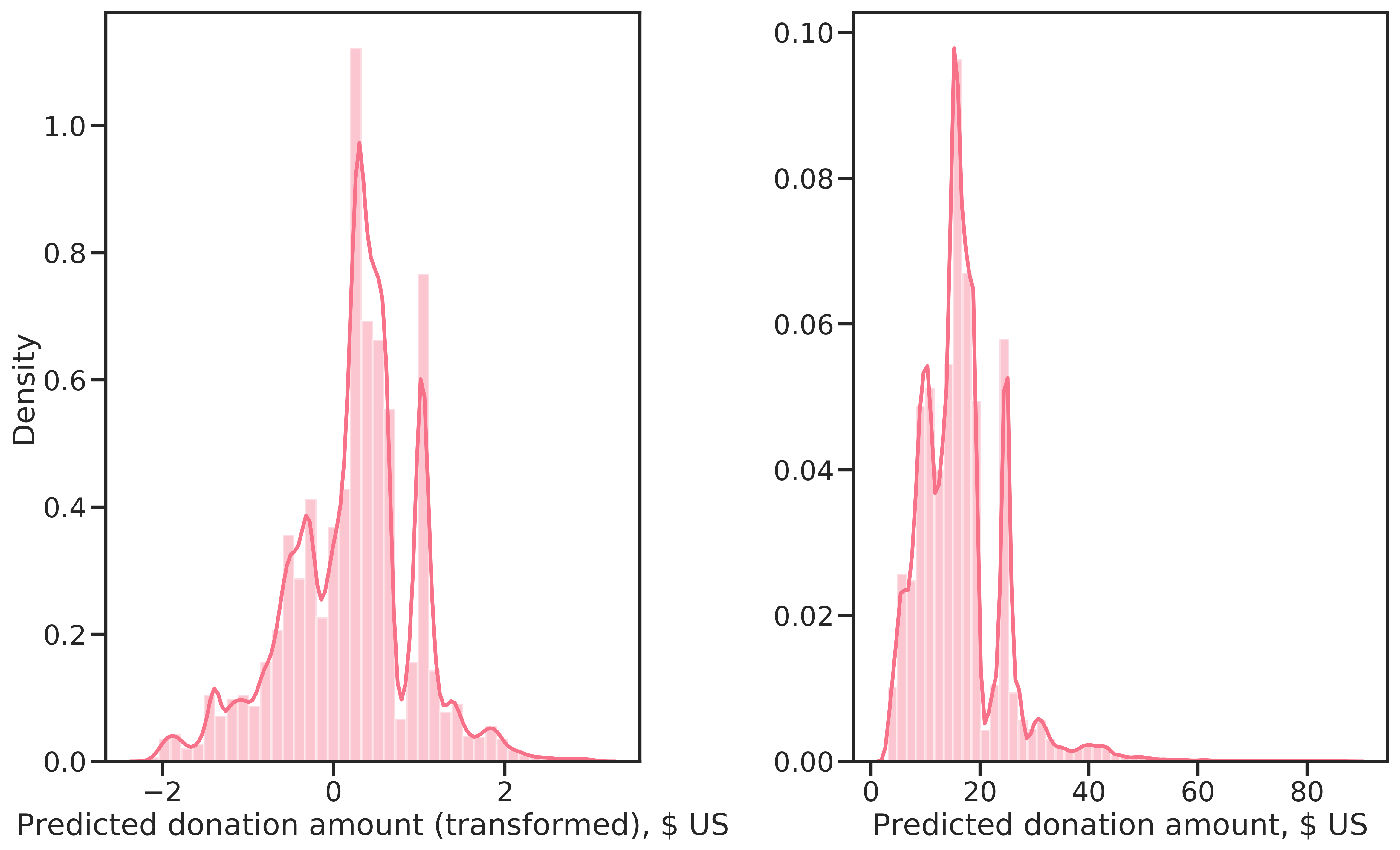
Figure 4.12: Conditionally predicted donation amounts, Box-Cox transformed (left) and on the original scale (right).

4.5.3 Profit Optimization

The correction factor $\alpha$, used to account for bias introduced by learning the regression models on a non-random sample, was found as described in section 3.4. First, estimated net profit $\hat{\Pi}$ was calculated using equation (2.4) for a grid of $\alpha$ values in $[0,1]$. Then, a cubic spline was fitted to the data and $\alpha$ optimized subsequently.

As can be observed in Figure 4.13, the region of $\alpha$ for high profit is narrow. This is not surprising given the distribution of $\hat{y}_d$ (Figure 4.12), which is narrowly concentrated around ~15 $. Furthermore, the curve is constant over much of the domain, meaning that all examples were selected from $\alpha \approx 0.15$. The cubic spline fits the data very well and finding the maximum at $\alpha^*=0.02$. For reference, a polynomial of degree 12 is also shown in 4.13, highlighting the difference in the fit for the two approaches.

$Expected profit for a range of $\alpha$ values in $[0,1]$ with overlayed cubic spline and polynomial function of order 12.$

Figure 4.13: Expected profit for a range of $\alpha$ values in $[0,1]$ with overlayed cubic spline and polynomial function of order 12.

4.5.4 Final Prediction

For the final prediction, an estimator combining the two-step prediction process was implemented in package kdd98. The estimator Kdd98ProfitEstimator was initialized with the GLMnet classifier and RF regressor determined as the best during model evaluation and selection.

Then, the estimator was fitted on the complete learning data set, thereby fitting both the classifier and regressor and optimizing $\alpha*$, which was computed as $\alpha^* = 0.023$.

The fitted estimator could then be used for prediction on the test data set. The results are shown in Table 4.1 together with the winners of the cup. The model learned in this thesis selects less donors compared to the top-ranked participants and has a higher mean donation amount. Nevertheless, net profit is lower, resulting in the $4^{th}$ rank.

The winner, Urban Science Applications with their proprietary software Gainsmarts, chose a two-step approach as well. In the first step, a logistic regression was used. The second step consisted of linear regression. Their software automated feature-engineering (by trying several different transformations for each feature) and feature selection through an expert system²¹. They selected a distinct subset of features for each step.

No information is available on SAS’s approach. Decisionhouse’s Quadstone on $3^{rd}$ rank also invested heavily in feature engineering. The proprietary software was specially designed for customer behavior modeling. They used decision trees for conditioned profit estimation using 6 features and an additive scorecard model for selecting examples based on 10 features in combination. For the estimation of donation amount, they also found the amount of the last donation and average donation amounts as important.

Surely, if domain knowledge had influenced feature engineering and feature selection for the model developed here, performance would have been better. Given the radically data-driven approach, the result can be considered good.

Table 4.1: Prediction results for the test data set (in color) and the results of the cup-winners. $N^*$ denotes number of examples selected. The theoretical maximum was calculated with: $ ($\sum_{i=1}^n \mathbb{1}_{\{\text{TARGET}_{D,i} > 0.0\}}*(\text{TARGET}_{D,i} - u)$ with $u$ the unit cost of 0.68 $ per mailing).
		Amount, $
	N*	Min	Mean	Std	Max	Net Profit	Percent of Maximum
GainSmarts	56330	-0.68	0.26	5.57	499.32	14712	20.22
SAS	55838	-0.68	0.26	5.64	499.32	14662	20.15
Quadstone	57836	-0.68	0.24	5.66	499.32	13954	19.17
Own	40984	-0.68	0.34	6.28	499.32	13877	19.07
CARRL	55650	-0.68	0.25	5.61	499.32	13825	19.00

However, these predictions were made using the true TARGET_D. When treating the data as unseen, predicted net profit was unrealistically high, at 861’562 $, which translates to an error of 6’208 %. In this case, net profit was calculated by substituting $(y_d-u)$ with $(\hat{y}_d-u)$ in Equation (2.4). However bad this result is, would the model developed be used to select examples for a promotion, it would still lead to relatively good net profit.