4.4 Model Evaluation and Selection

Model evaluation and -selection may be studied in detail in notebook 6_Model_Evaluation_Selection.ipynb¹⁹. As will be explained below, all classifiers performed rather weak and were highly influenced by the imbalance in the data. The best results were achieved when using SMOTE resampling. Random over-/undersampling and specifying class weights had an inferior effect on model performance.

Among the classifiers evaluated, GLMnet showed the best performance and was thus chosen.

For the regression models, RF outperformed the other models, although the differences were less pronounced compared to the classifier results.

4.4.1 Classifiers

During grid search, models were trained individually for best F1 and recall. The models trained for high recall had only slightly worse precision than those trained for high F1, but at the same time better recall scores (see Jupyter notebook 6_Model_Evaluation_Selection.ipynb). Therefore, the recall-trained models were considered for selection of the classifier.

Evaluation was based on the recall scores, confusion matrices, receiver operating characteristic (ROC) indicating model performance through an area under the curve score (ROC-AUC) and precision-recall (PR) curves.

If only the recall score were considered, the decision would be obvious, as shown in Figure 4.2. SVM has ~74 % recall, with the next-best scores at 54 % and 53 %. However, it is important to also consider the false positives as those cost money and decrease net profit.

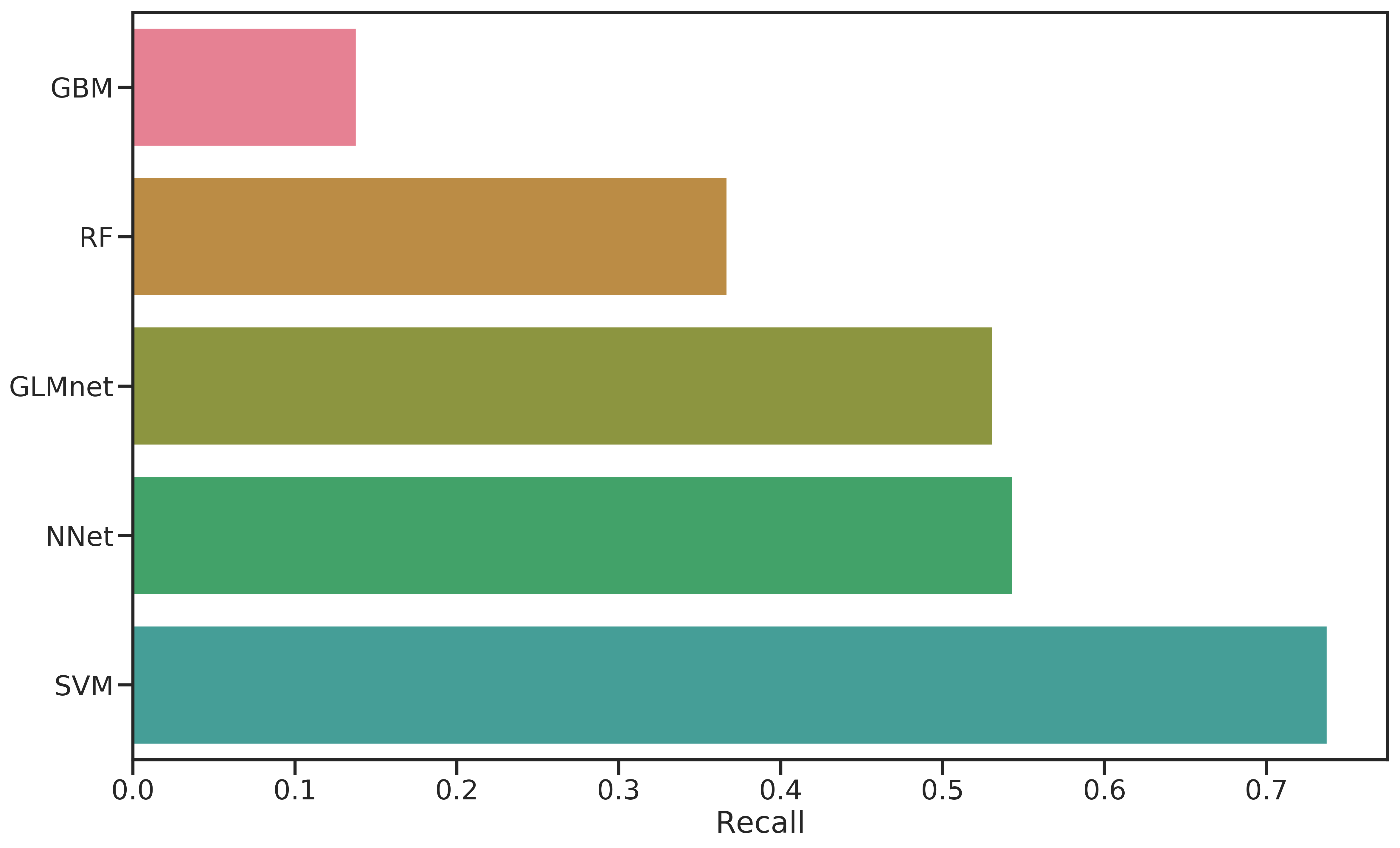
Figure 4.2: Comparison of recall scores for all classifiers evaluated.

The ROC-AUC curve (Figure 4.3, left panel) was constructed by evaluating the false positive rate (FPR) against the true positive rate (TPR) at various thresholds for the predicted class probabilities of examples in the training data. The closer the curve is to the top-left corner, the better a model performs (large TPR and at the same time a low FPR for a wide range of thresholds). All classifiers seemingly performed rather weak. In the case of imbalanced data, the majority class dominates this metric. The false positive rate is $FPR = \frac{FP}{FP+TN}$. This means that as the false positives (FP) decrease due to an increasing threshold, FPR does not change a lot.

The PR curve with precision $P = \frac{TP}{TP+FP}$ plotted against recall $R = \frac{TP}{{TP+FN}}$ at different threshold values is sensitive to false positives and, since TN is not involved, better suited for the imbalanced data at hand. To construct the curve, recall is plotted against precision for various threshold values of the predicted class probabilities. For good models, the curve is close to the top-right corner. The right panel of Figure 4.3 shows the models in direct comparison. All of them suffer from low precision except for the highest threshold values. Again, this is caused by the high imbalance in the data.

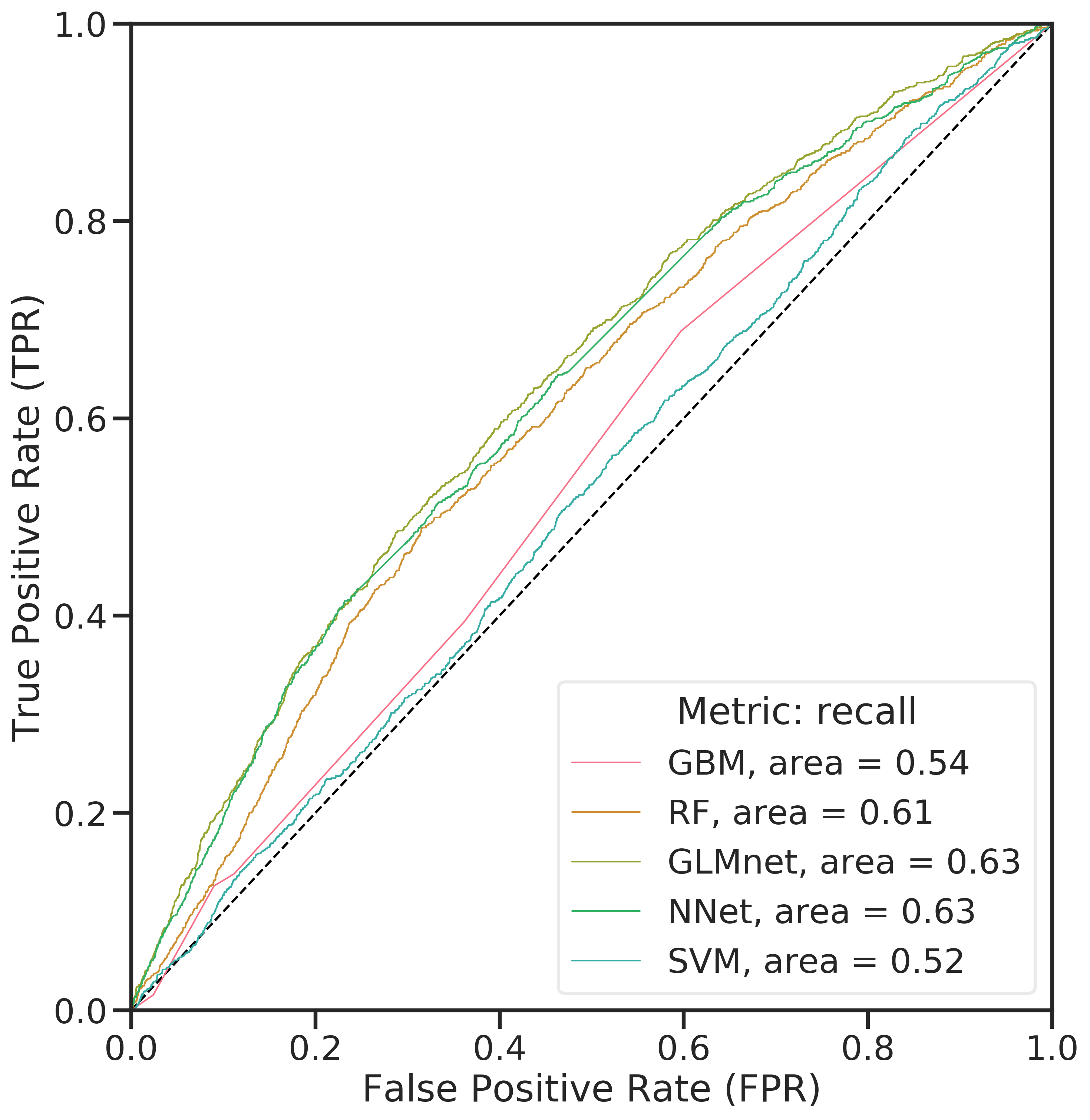
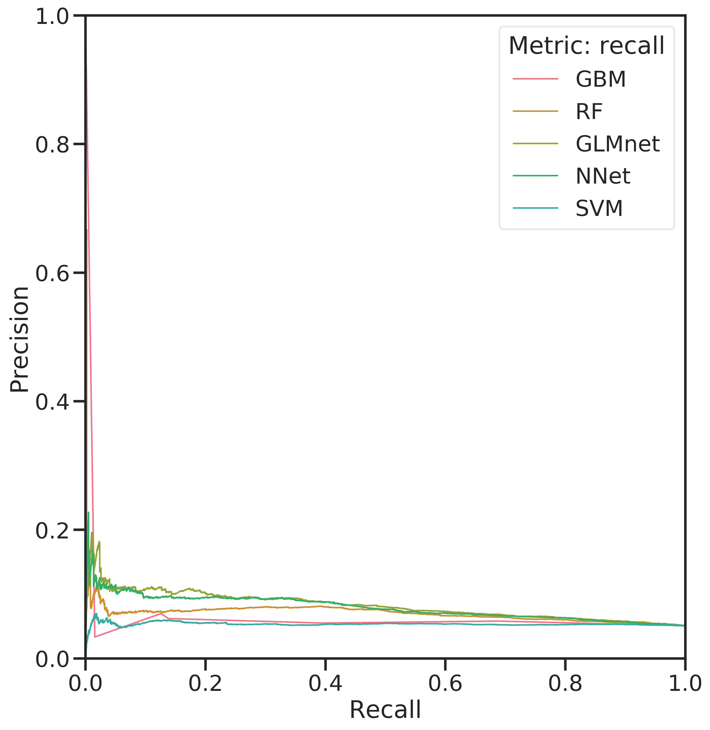
Figure 4.3: Comparison of ROC-AUC for the evaluated classifiers (left) and PR curves (right) for the classifiers.

More insight can be gained from the confusion matrices, shown in Figure 4.4. The best classifier should have a high recall, predicting many donors correctly, and at the same time a low False Positive Rate (FPR).

From the confusion matrices, it becomes obvious that for SVM, the trade off for high recall is also a high FPR. The false positives can be directly translated to cost: the 12’985 false positives in this case would amount to 8’830 $ at a unit cost of 0.68 $, while the 715 true positives generate an expected profit of only 8’808 $ (with a mean net profit of 12.32 $).

Evidently, GLMnet an NNet have a relatively good balance of recall and FPR. GBM performs well for FPR, which means less money lost due to unit costs, but has a very low recall.

GLMnet and NNet were also combined into a voting classifier. This classifier creates an ensemble that predicts through a majority vote, therefore compensating for the individual classifier’s weaknesses. It exhibits a slightly lower recall for a slight decrease in FPR. Since recall was seen as being more important, it was not investigated further.

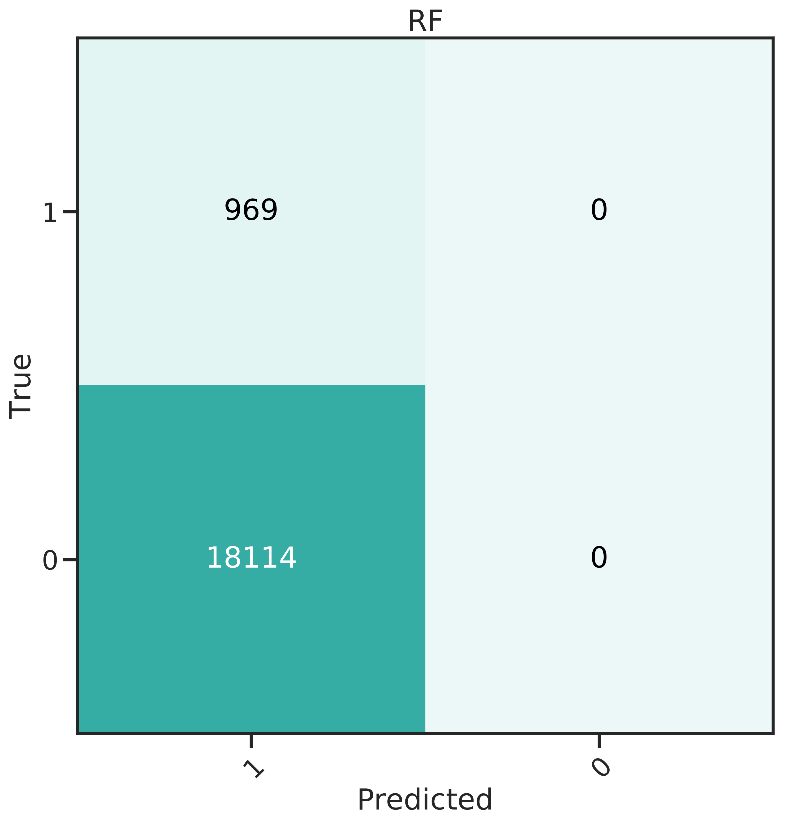
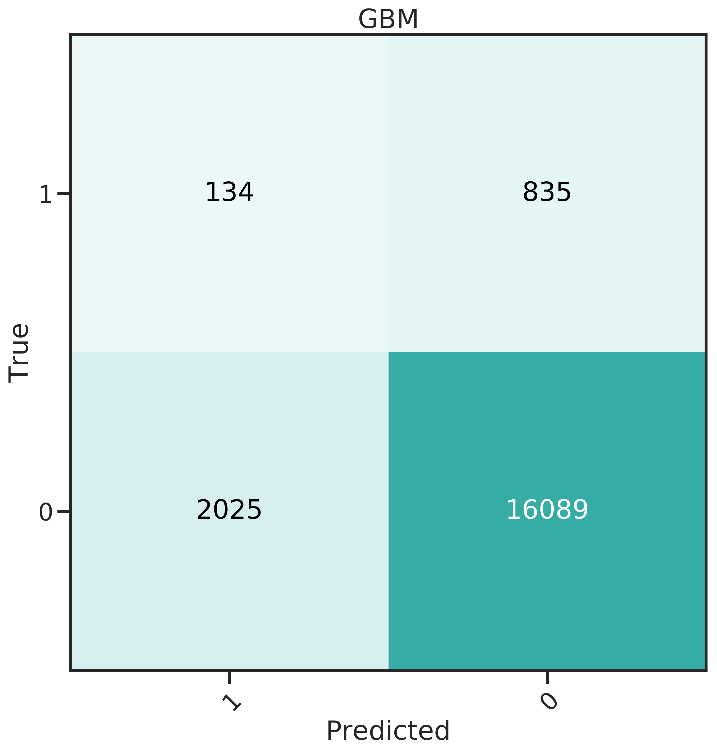
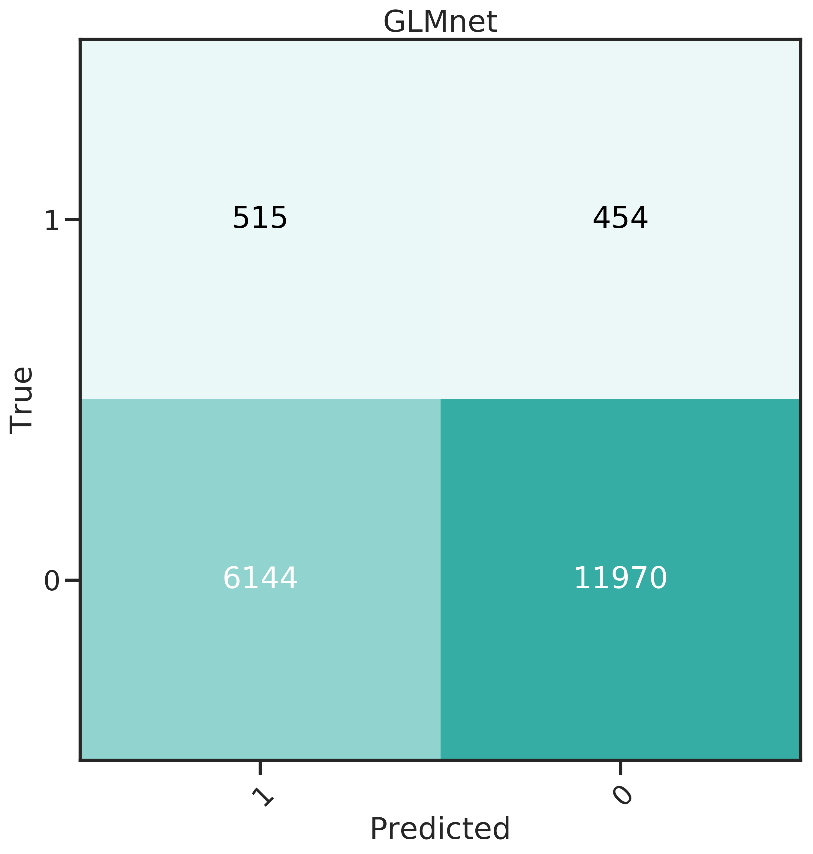
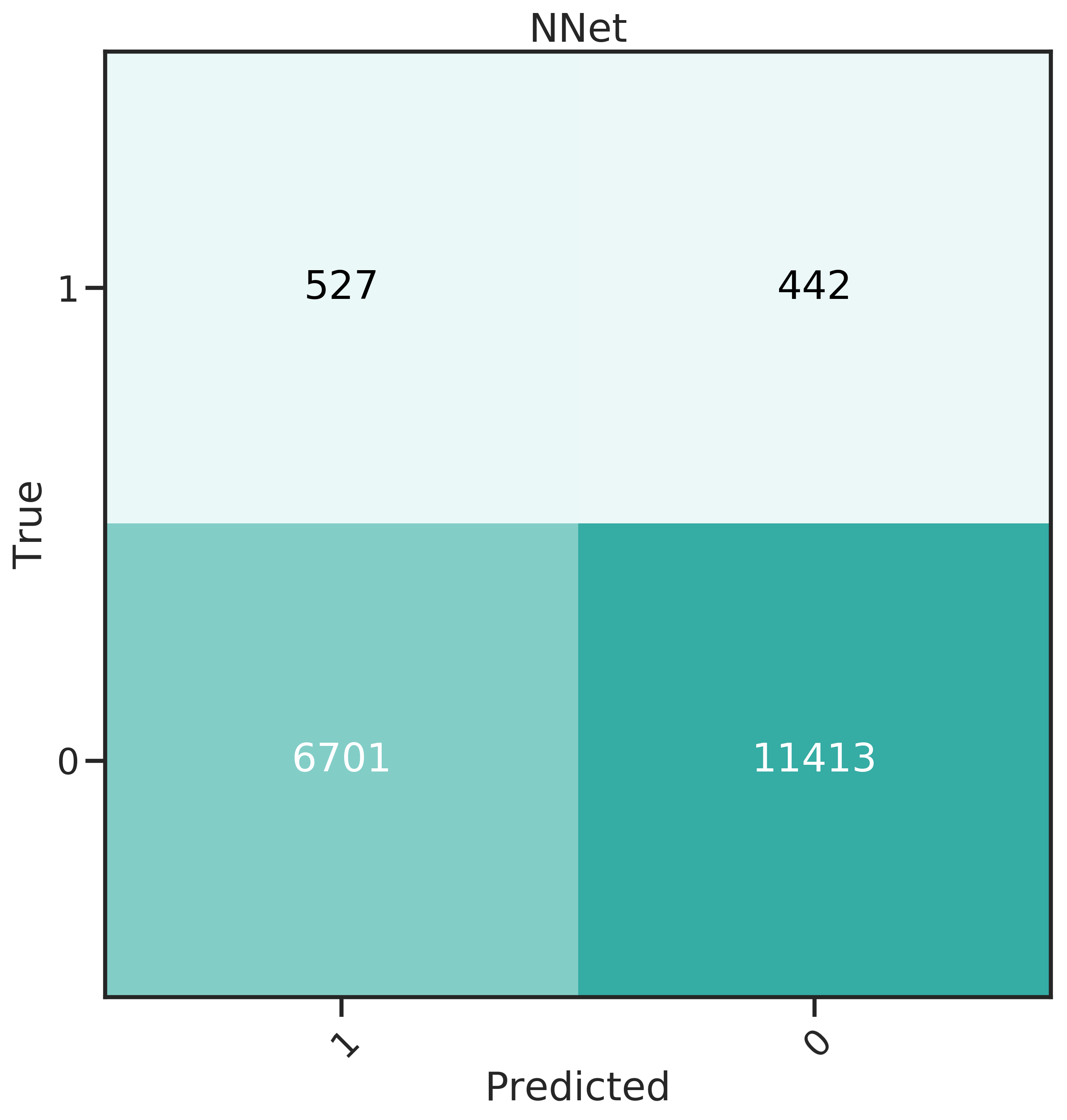
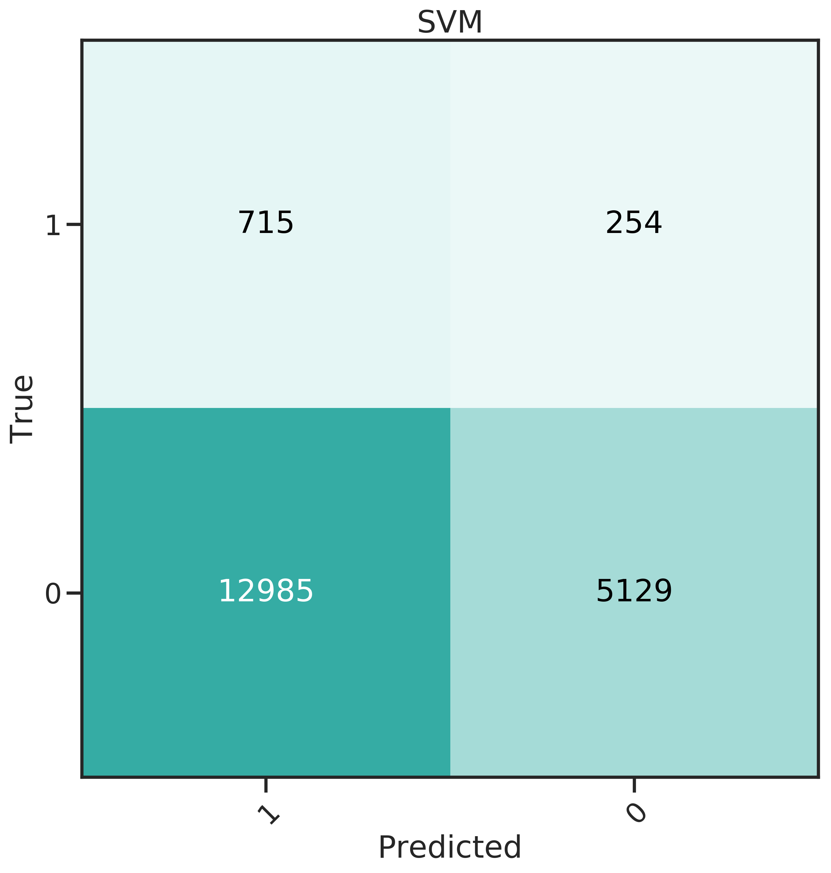
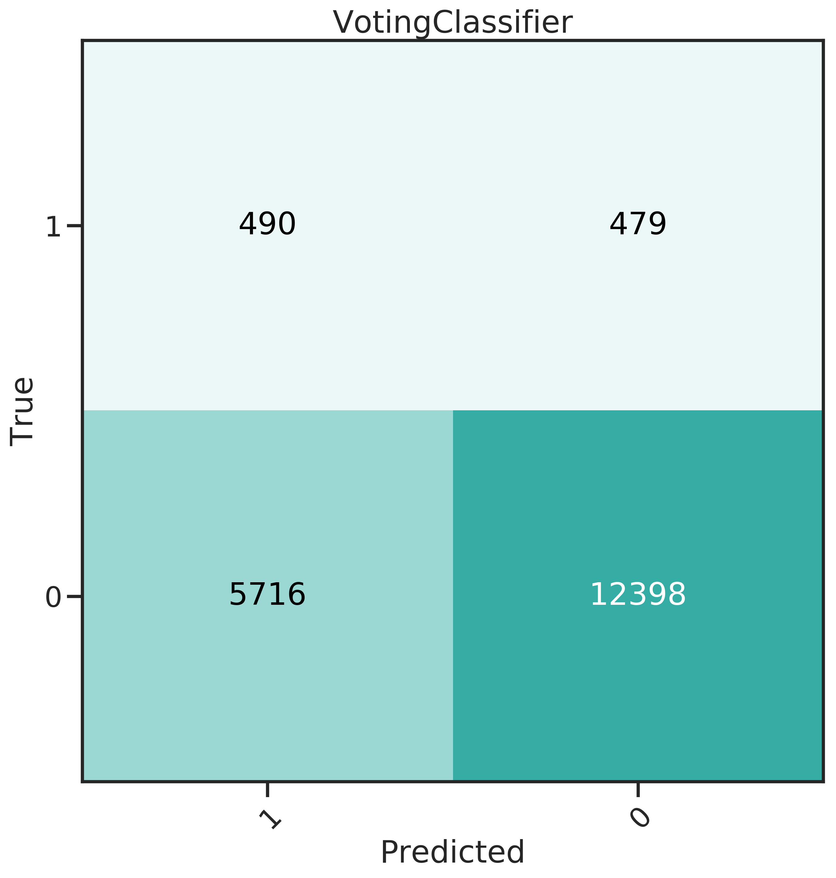
Confusion matrices for the 6 classifiers studied.

Figure 4.4: Confusion matrices for the 6 classifiers studied.

The non-null coefficients of the GLMnet model are shown in 4.5. 22 coefficients are non-null. The absolute values of the coefficients indicate importance of the respective feature. The first five features are from the promotion- and giving history and are concerned with the amount and frequency of donations.

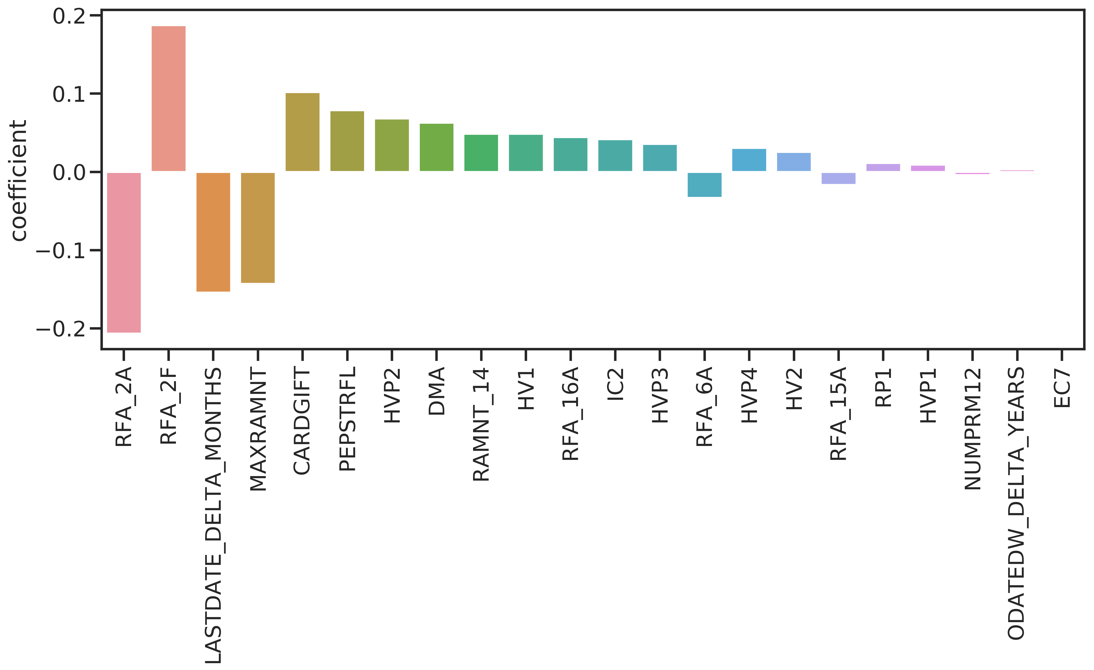
Figure 4.5: Coefficient values for GLMnet.

Although RF performed poorly, it can be used to have a second source of information on the important features. The measure implemented in scikit-learn is the Gini importance as described in Breiman et al. (1984). It represents the total decrease in impurity (see Section 3.5.4.1) due to nodes split on feature $f$, averaged over all trees in the forest. The most important features again are all from the giving history, followed by the promotion history. US census features are not important (see Figure 4.6).

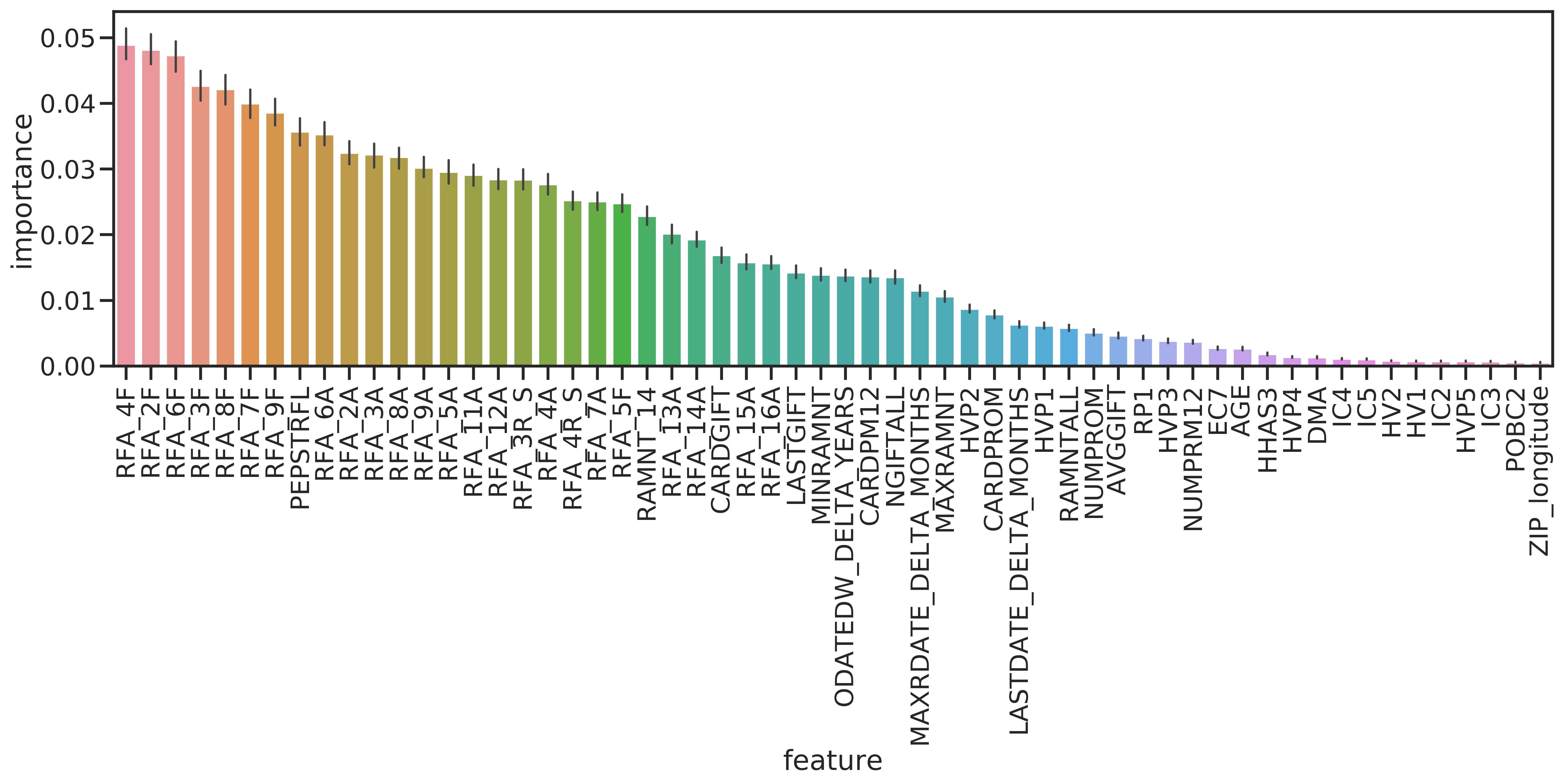
Feature importances determined with the RF classifier. Impurity is measured by Gini importance / mean decrease impurity. Error bars give bootstrap error on 50 repetitions.

Figure 4.6: Feature importances determined with the RF classifier. Impurity is measured by Gini importance / mean decrease impurity. Error bars give bootstrap error on 50 repetitions.

4.4.2 Regressors

As explained in Section 3.4, the regressors were learned on a subset of the training data comprised of all donors: $\{\{x_i, y_i\}|y_{b,i} = 1\}$. Before learning, TARGET_D was Box-Cox transformed for normalization with $\lambda=0.0239$. The goal of the transformation was to improve regression models’ performance. The transformed data somewhat resembles a normal distribution, although there are several modes to be made out (see Figure 4.7).

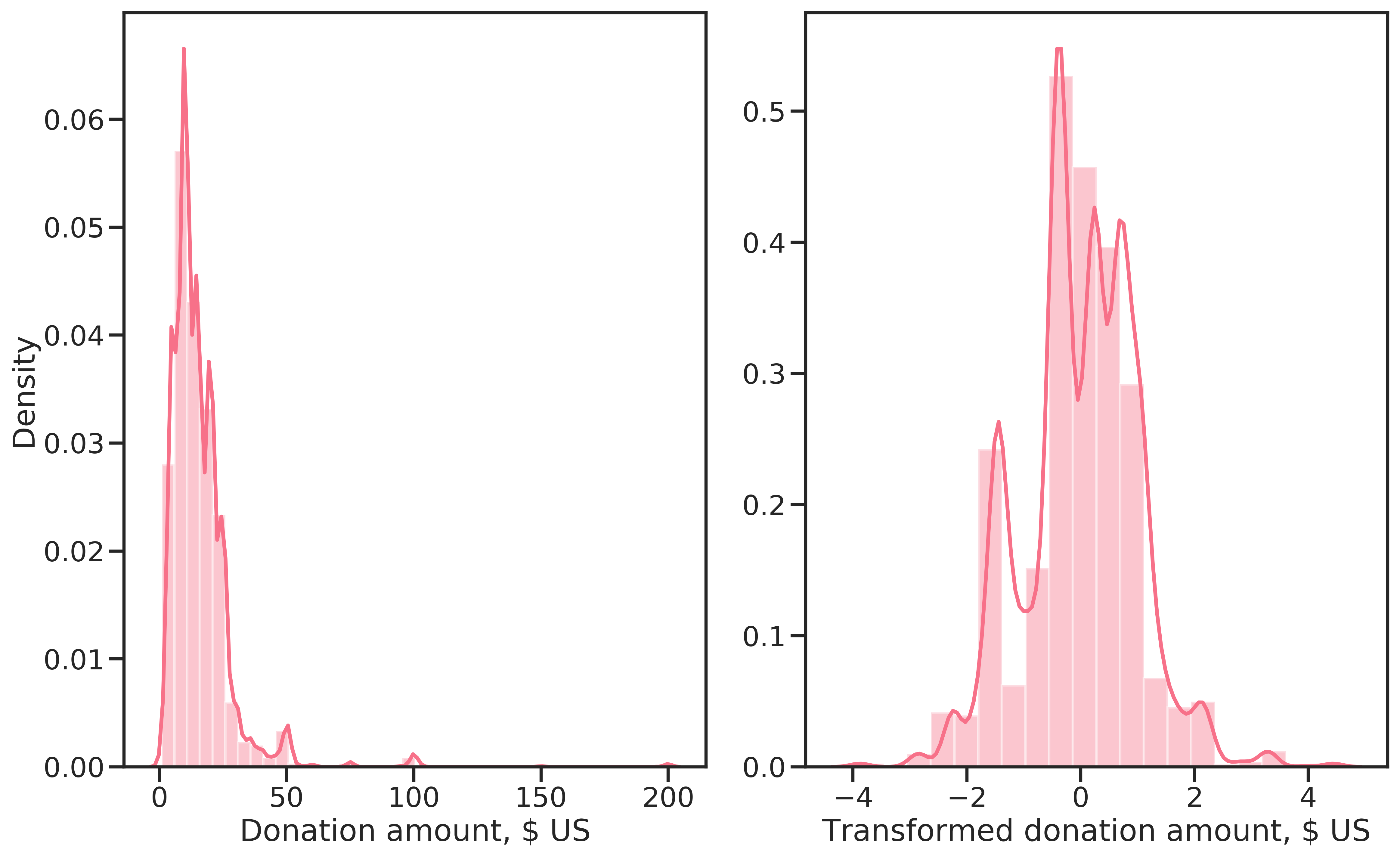
Figure 4.7: Target before transformation (left) and after a Box-Cox transformation (right).

The resulting distribution of predicted donation amounts on the training data is shown in Figure 4.8. Except for SVR, the models produce very similar results. Again, the multi-modal distribution is found (refer to Figure 4.7). RF and SVR are relatively symmetric, while BR and ElasticNet produce right-skewed distributions that predict very large donation amounts for some examples.

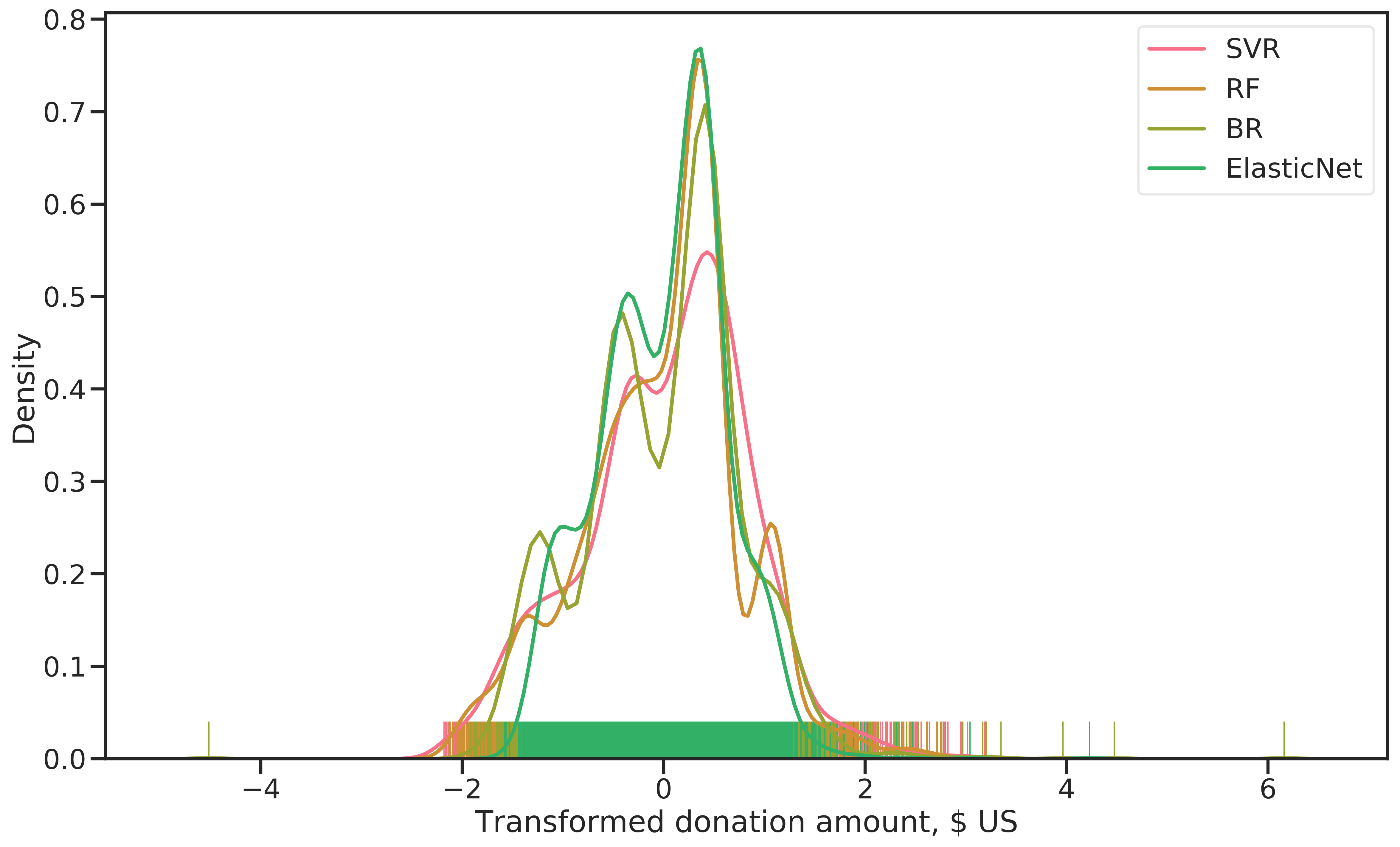
Figure 4.8: Distribution of (Box-Cox transformed) donation amounts for the four regressors evaluated.

The regressor for final prediction was selected by $R^2$ score on a test set (20% of the learning data was used). RF was the best performing model with $R^2 = 0.72$ (see Figure 4.9).

$Evaluation metric $R^2$ for all regression models evaluated. The domain for $R^2$ is $(-\inf, 1]$.)$

Figure 4.9: Evaluation metric $R^2$ for all regression models evaluated. The domain for $R^2$ is $(-\inf, 1]$.)

Again, RF enables to interpret the importance of features. The results (Figure 4.10) show that mainly the amount of the last donation, and to a lesser amount the average donation amount and the amounts of the last three donations were important for predicting donation amounts. This would indicate that donors tend to always donate the same sums.

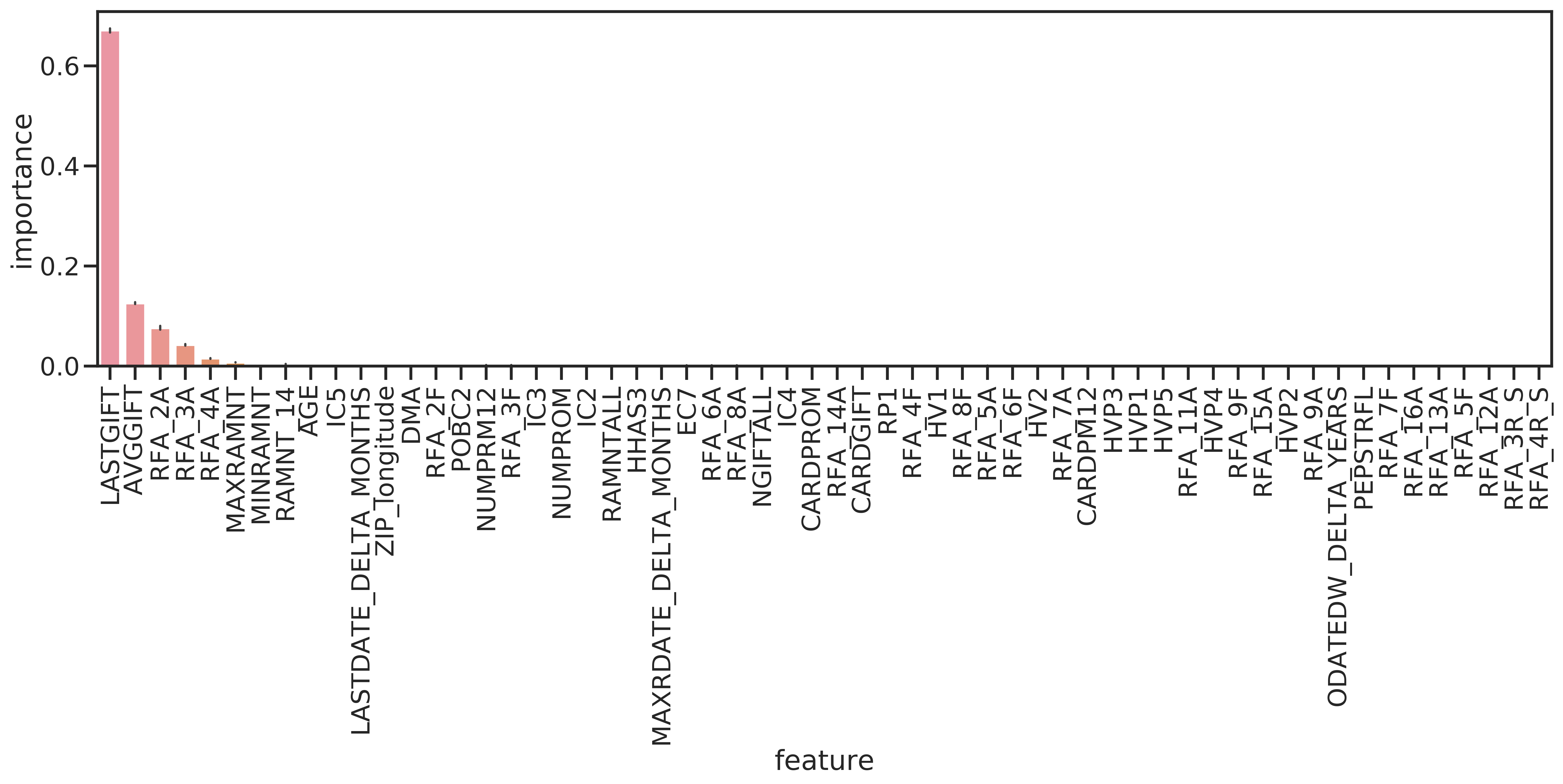
Figure 4.10: Feature importances for the RF regressor.

https://github.com/datarian/thesis-msc-statistics/tree/master/code/notebooks/6_Model_Evaluation_Selection.ipynb ↩